Learning some R #3

Carrying on from last night: I could’t get the separating hyperplane (aka decision line) to draw with this code:

Apparently, the sample codes in git for chapter 2 do work. So what went wrong??!

heights.weights <- transform(heights.weights,
                             Male = ifelse(Gender == 'Male', 1, 0))

logit.model <- glm(Male ~ Weight + Height,
                   data = heights.weights,
                   family = binomial(link = 'logit'))

ggplot(heights.weights, aes(x = Height, y = Weight)) +
  geom_point(aes(color = Gender, alpha = 0.25)) +
  scale_alpha(guide = "none") + 
  scale_color_manual(values = c("Male" = "black", "Female" = "gray")) +
  theme_bw() +
  stat_abline(intercept = -coef(logit.model)[1] / coef(logit.model)[2],
              slope = - coef(logit.model)[3] / coef(logit.model)[2],
              geom = 'abline',
              color = 'black')

Seems that I wrote the logit.model part wrongly. Correcting the order for the Male ~ Weight + Height part did the trick.

heights.weights <- transform(heights.weights,
                             Male = ifelse(Gender == 'Male', 1, 0))

logit.model <- glm(Male ~ Weight + Height,
                   data = heights.weights,
                   family = binomial(link = 'logit'))

ggplot(heights.weights, aes(x = Height, y = Weight, color = Gender)) +
    geom_point() +
    stat_abline(intercept = - coef(logit.model)[1] / coef(logit.model)[2],
                slope = - coef(logit.model)[3] / coef(logit.model)[2],
                geom = 'abline', color = 'black')

Dissecting the transform command a little, how DOES it work?

> heights.weights[1:10,]
   Gender   Height   Weight
1    Male 73.84702 241.8936
2    Male 68.78190 162.3105
3    Male 74.11011 212.7409
4    Male 71.73098 220.0425
5    Male 69.88180 206.3498
6    Male 67.25302 152.2122
7    Male 68.78508 183.9279
8    Male 68.34852 167.9711
9    Male 67.01895 175.9294
10   Male 63.45649 156.3997

> heights.weights <- transform(heights.weights,
+                              Male = ifelse(Gender == 'Male', 1, 0))

> heights.weights[1:10,]
   Gender   Height   Weight Male
1    Male 73.84702 241.8936    1
2    Male 68.78190 162.3105    1
3    Male 74.11011 212.7409    1
4    Male 71.73098 220.0425    1
5    Male 69.88180 206.3498    1
6    Male 67.25302 152.2122    1
7    Male 68.78508 183.9279    1
8    Male 68.34852 167.9711    1
9    Male 67.01895 175.9294    1
10   Male 63.45649 156.3997    1

Ok, so it just created a column (“tag”) which is populated according to the contents of the first column (a factor, or categories).

With this, the glm command (generalized linear models) command makes more sense, though I still have little-to-no idea what the parameters mean even after reading the help pages…

Anyway, onwards to chapter 3, binary classification! We’ll see if there’s a need to learn glm in-depth by myself later.

Learning some R #2

Continuing my scratchpad post on the R language as I go through ML for Hackers:

Sub-selection looks similar to other languages like those used in MATLAB:

> heights.weights[1:20,]
   Gender   Height   Weight
1    Male 73.84702 241.8936
2    Male 68.78190 162.3105
3    Male 74.11011 212.7409
4    Male 71.73098 220.0425
5    Male 69.88180 206.3498
6    Male 67.25302 152.2122
7    Male 68.78508 183.9279
8    Male 68.34852 167.9711
9    Male 67.01895 175.9294
10   Male 63.45649 156.3997
11   Male 71.19538 186.6049
12   Male 71.64081 213.7412
13   Male 64.76633 167.1275
14   Male 69.28307 189.4462
15   Male 69.24373 186.4342
16   Male 67.64562 172.1869
17   Male 72.41832 196.0285
18   Male 63.97433 172.8835
19   Male 69.64006 185.9840
20   Male 67.93600 182.4266
> heights.weights[1:20,1]
 [1] Male Male Male Male Male Male Male Male Male Male Male Male Male Male Male
[16] Male Male Male Male Male
Levels: Female Male
> heights.weights[1:20,2]
 [1] 73.84702 68.78190 74.11011 71.73098 69.88180 67.25302 68.78508 68.34852
 [9] 67.01895 63.45649 71.19538 71.64081 64.76633 69.28307 69.24373 67.64562
[17] 72.41832 63.97433 69.64006 67.93600
> heights.weights[1:20,3]
 [1] 241.8936 162.3105 212.7409 220.0425 206.3498 152.2122 183.9279 167.9711
 [9] 175.9294 156.3997 186.6049 213.7412 167.1275 189.4462 186.4342 172.1869
[17] 196.0285 172.8835 185.9840 182.4266

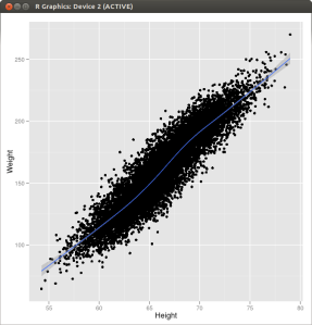
First scatterplot: done by defining the second axis in the aesthetics function.

> ggplot(heights.weights, aes(x = Height, y = Weight)) + geom_point()

Plotting a linear estimate is simply a matter of adding in the geom_smooth() function to the line. I’m starting to really like the way visualization of table data is done here 🙂

> ggplot(heights.weights, aes(x = Height, y = Weight)) + geom_point() + geom_smooth()

Splitting the data points by gender into two groups:

> ggplot(heights.weights, aes(x = Height, y = Weight, color = Gender)) + geom_point()

Couldn’t get the “separating hyperplane” (decision line) draw on the plot though…will need to see what went wrong there when I resume.

> heights.weights <- transform(heights.weights, 
+                              Male = ifelse(Gender == 'Male', 1, 0))
> logit.model <- glm(Male ~ Height + Weight, 
+                    data = heights.weights, 
+                    family = binomial(link = 'logit'))
> ggplot(heights.weights, aes(x = Height, y = Weight, color = Gender)) + 
+   geom_point() + 
+   stat_abline(intercept = - coef(logit.model)[1] / coef(logit.model)[2], 
+               slope = - coef(logit.model)[3] / coef(logit.model)[2], 
+               geom = 'abline', color = 'black')

Learning some R

Just trying out some of the stuff on R programming as I read Machine Learning for Hackers by Drew Conway and John Myles White. The data and source codes can be found at https://github.com/johnmyleswhite/ML_for_Hackers (thanks @ericnovik)

The first chapter on “Using R” was a little too hard to follow for a R beginner like me, so I decided to learn the concepts and terms from chapter 2 (Data Exploration) first and get back to chapter 1 as needed.